Chapter I

Capital Markets and Investment Performance

Returns, risk measurement, the equity premium, and historical capital markets data.

Overview

Securities are contractual promises of future payment or delivery, standardized so that they can be traded on exchanges. There are three main types of financial security: bonds, which promise fixed future payments; stocks, which promise a future, unspecified stream of dividends; and derivative contracts, which specify a payment or the delivery of a security contingent on future events.

Key Concept

All securities, no matter how complex, share one essential feature: they are economic claims against future benefits, and therefore always incorporate a time dimension.

Capital Market History

The first bond market began in Venice, where from the twelfth century the Republic raised money from its citizens through forced loans in return for future repayment with interest. In 1262 these loans were consolidated into a single funded debt, the Monte Vecchio, whose shares — the prestiti — paid 5% annual interest and changed hands in the Rialto marketplace. It was the first true secondary market in a government security.

The earliest corporations emerged in fourteenth-century Toulouse, where investors held and traded shares in large-scale milling companies, collecting dividends that varied with the firm’s profits.

Engraving of the mills of the Bazacle on the Garonne at Toulouse — The mills of the Bazacle on the Garonne at Toulouse. Shares in the milling company were held, traded, and paid dividends from the fourteenth century — among the earliest true corporations.

Seventeenth-century view of the courtyard of the Amsterdam Beurs — The courtyard of the Amsterdam Beurs, Hendrick de Keyser’s exchange. The shares of the Dutch East India Company traded here — the world’s first active stock market.

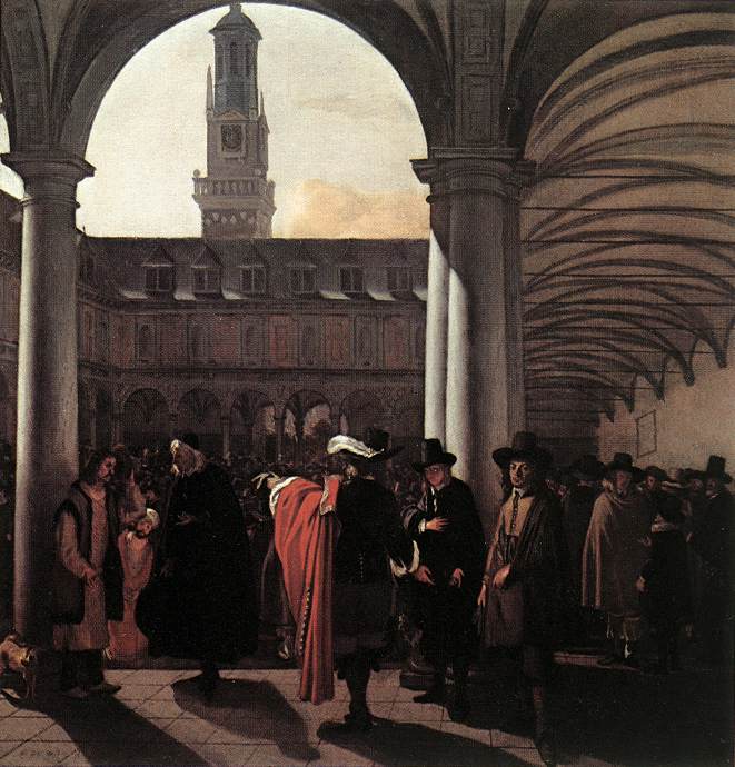
Amsterdam was the first active stock market: the Dutch East India Company was a national enterprise with hundreds of shareholders and busy speculators. It also issued tradable bonds — the first corporation to do so — and Amsterdam is the likely birthplace of traded options, the derivatives that give their owner the right to buy or sell shares of stock.

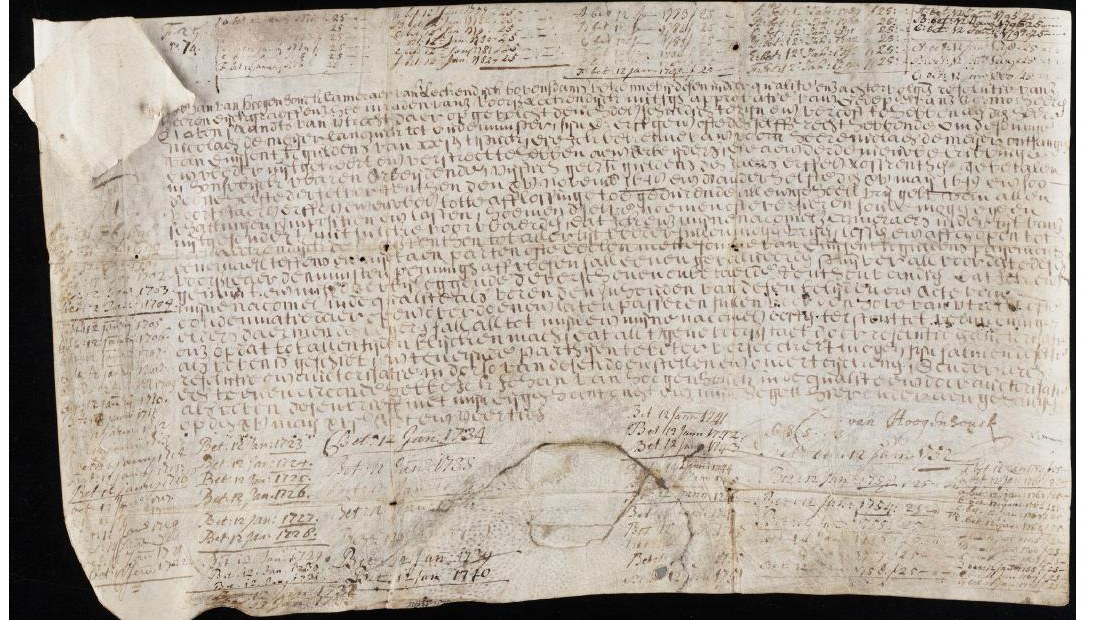
These early securities could endure for centuries. A perpetual bond issued in 1648 by the Lekdijk Bovendams water authority in the Netherlands — now among the treasures of Yale’s Beinecke Library — has its margins covered with interest payments recorded over hundreds of years, and it is honored still.

The 1648 Lekdijk Bovendams perpetual bond, with centuries of interest payments noted in the margins — The 1648 Lekdijk Bovendams perpetuity (Yale, Beinecke Library). The marginal notes are centuries of interest payments — a bond still paying nearly four hundred years on.

Most securities traded before the nineteenth century were bonds, typically issued by governments. But the first widespread stock-market bubble swept Europe in 1719 and 1720. Variously called the South Sea Bubble, the Mississippi Bubble, or the Dutch Windhandel, it was sparked by speculation in Atlantic trade and by promising new technologies and financial innovations at the dawn of the Industrial Revolution.

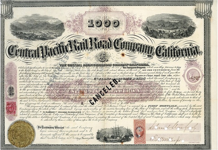
An ornate 1867 Central Pacific Railroad $1,000 gold bond certificate — A Central Pacific Railroad $1,000 first-mortgage gold bond of 1867, signed by Leland Stanford as president. Bonds like this financed the American transcontinental railroad. (Wikimedia Commons, CC0.)

The modern era of capital markets dates to the late nineteenth century, spurred by the global expansion of railroads, which demanded massive capital investment. Nations and corporations turned to the stock and bond markets to finance large-scale infrastructure — and expensive wars. London was the dominant marketplace of the nineteenth century, alongside a constellation of European exchanges in Paris, Brussels, Berlin, and Saint Petersburg. American markets overtook those of Europe in the twentieth century, and much of what we know about the risk and return of stocks, bonds, and options comes from records of American marketplaces — the New York Stock Exchange and the Chicago Board Options Exchange.

The global expansion of finance in the twenty-first century, particularly in India and China, has vastly enlarged the supply of capital, increased the number of investors enormously, and afforded all investors the opportunity to diversify globally. The tools we explore in this text are the foundation of the decisions those investors face.

One long pattern runs beneath all of this history. Across seven centuries, the real return on safe lending has drifted steadily downward — a decline visible only at the scale of centuries, and one of the most striking regularities in financial history.

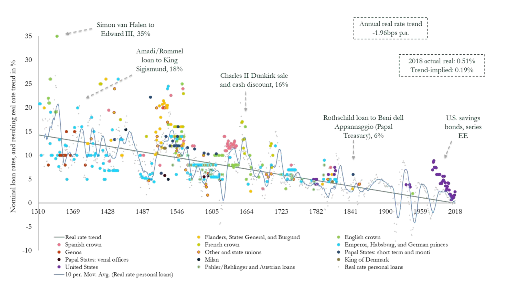
Nominal interest rates on loans to sovereigns, 1310 to 2018, each point a loan colored by lender, with the fitted real-rate trend falling about two basis points a year from double digits toward near zero

Seven centuries of real interest rates. Nominal interest rates on loans to sovereigns from 1310 to 2018 — each point a loan, colored by lender — with the fitted real-rate trend running through them. Paul Schmelzing dates this “suprasecular” decline at roughly two basis points a year: real rates fall from the double digits of the late medieval period toward the near-zero levels of today (0.51% in 2018), with wide swings around the trend. Figure from Paul Schmelzing, The Long Run (Yale University Press, forthcoming); see also “Eight Centuries of Global Real Interest Rates, R−G, and the Suprasecular Decline, 1311–2018,” Bank of England Staff Working Paper No. 845 (2020).

Investing Today

Bring the story to the present. How large is investment in the world now? A clean way to see it is as a share of what the world produces. Each year humankind does not consume everything it makes; it sets a portion aside — building factories, housing, machinery, and infrastructure, and creating the financial claims that fund them. Economists call this gross capital formation, and for the world as a whole it runs at roughly a quarter of global output, year after year. The figure below is drawn live from the World Bank, so it stays current as new data arrive.

Loading the latest World Bank figure…

Figure 1.1. How much of the world’s output is invested. Of everything the world produces each year, the share directed to new capital rather than consumed — factories, housing, infrastructure, and the financial assets that fund them — is its gross capital formation. For the world it has held near a quarter of GDP for decades. This figure is drawn live from the World Bank, so the latest reading updates itself as new data are published.

This flow of saving collects in a handful of large pools. Norway’s Government Pension Fund Global, built from the nation’s North Sea oil, holds on the order of two trillion dollars and owns, on average, about 1.5% of every listed company on earth. Japan’s Government Pension Investment Fund is comparable in scale. Private asset managers are larger still: BlackRock and Vanguard each invest on the order of ten trillion dollars or more on behalf of millions of ordinary savers. University endowments — Harvard’s and Yale’s among the largest — are managed to sustain their institutions in perpetuity. Different as their mandates are, in each case the task is the same: present assets arranged to meet future needs. That is the investor’s problem, and it is the subject of this book. (Fund figures as of 2024–2025.)

I. Time and Money

Almost everything in this book comes back to one basic observation: a dollar today is worth more than a dollar tomorrow. Offer someone a dollar now or the same dollar in a year and they take it now — and they are right to. A dollar in hand can be put to work and grow; a dollar merely promised must be waited for, and the wait is neither free nor certain. This is the time value of money, and learning to compare sums that arrive at different times is the first skill of finance.

The idea takes a moment to grasp, and it helps to see that it runs in both directions at once. Suppose money can be invested to earn an interest rate $r$. Then:

If I lend you a dollar today, I give up the growth it would have earned — so to make me whole, you must repay more than a dollar next year. At a rate $r$, you owe me $1+r$.
And if you promise to pay me a dollar a year from now, that promise is worth less than a dollar today — because I could instead hold a dollar now and grow it myself. To value the promise I run the growth backwards, or discount it: a dollar next year is worth $1/(1+r)$ today.

The two are the same relationship seen from opposite ends: compounding grows a sum over time, and discounting reverses that growth to find its value today. The amount a future payment is worth today is its present value:

Present Value of a One-Period Cash Flow

$$PV=\frac{C}{1+r}$$

where $C$ is the cash to be received next period and $r$ is the interest rate. At a rate of 5%, a dollar due next year is worth about ninety-five cents today ($1/1.05 \approx 0.95$). You would rationally part with about ninety-five cents now for a sound promise of a dollar in a year — and the higher the rate, the less you would pay, because the more your own money could have grown while you waited.

Many Periods: The Exponential Curve

Stretch the wait to many years and the logic compounds. A dollar today grows to $(1+r)^t$ after $t$ years, so a dollar promised $t$ years out is worth $1/(1+r)^t$ today. Both are exponential curves — one rising, one falling — and they are the same curve traced in opposite directions. Set the rate below and watch either one: how a dollar grows if you invest it, or how little a distant dollar is worth if you must wait for it.

One of the Six · Picture 1 — Compound Growth

Interest rate r: 6.0% Horizon: 20 years log scale

Figure 1.2. The value of money across time. Set the interest rate and slide the horizon. In its default view the curve shows what a single future dollar is worth today: it begins at a full dollar now and decays toward nothing the farther off the payment lies — and the higher the rate, the faster it falls. Flip the switch to run the same exponential forward, and it becomes the compound-growth curve, what a dollar invested today becomes. Tick log scale and the exponential straightens into a line whose slope is the rate itself. Discounting and growing are one curve traced in two directions.

How you use it

Use this curve to put money from different dates on equal footing. Before you compare, price, or decide, pull every future sum back to today's dollars by discounting it down this curve — a distant payment is worth its height on the falling line, not its face value. Every valuation in the book begins here.

The four lenses for reading each picture ↗

This is not a modern picture, and the question behind it was not a modern question. Jakob Bernoulli asked what becomes of a loan when the interest is credited not once a year, nor quarterly, nor daily, but at every instant — the year cut into moments innumera aequalia, innumerably many and all equal. It reads like a scholastic exercise about slicing time into nothing. Its answer was a new number.

Bernoulli showed the amount cannot run away. However finely the year is divided, a sum lent for a year at 100% does not grow without bound: it converges, and the limit lies between 2 and 3.¹ That limit is e, the base of the natural logarithm, and Bernoulli reached it by way of a lending problem — not through geometry, not through quadrature, but by asking what a creditor is owed. Euler would not give the number a name for another four decades.

The abstraction turned out to be literal. Continuous compounding is no longer a thought experiment about infinitesimal slices of a year: it is how money is priced. It is the force of interest in an actuarial table, the drift in a diffusion, the instantaneous rate sitting underneath every option formula on a modern desk. What Bernoulli proposed as a limiting case is the assumption that quantitative finance now runs on as a matter of course.

And he drew it. The result appears in the Tractatus de seriebus infinitis, bound with his posthumous Ars Conjectandi of 1713, and what is rarely noticed is that the argument is stated as a figure. The Scholium reads as instructions for reading a plate, and the plate is there.

He sets the principal as an ordinate, BC = 1. The year runs along the axis as BI, “divided at the points E, F, G, &c. into innumerably many equal moments.” At each moment the sum is struck again, giving the ordinates EK, FL, GM — and because the moments are equal, those ordinates stand in continued proportion. The last ordinate, IO, “will denote the value of what is owed to the creditor when the whole year has elapsed.”

Jakob Bernoulli's Figure 1 of 1713: a logarithmic curve above an axis, with ordinates rising from the points B, E, F, G, R, I to the curve at C, K, L, M, N, O

The year — BI The principal — BC = 1 The moments — E, F, G Struck again — EK, FL, GM, RN The year’s end — IO The curve

Tap a label — or the engraving itself — to pick the construction out of the plate.

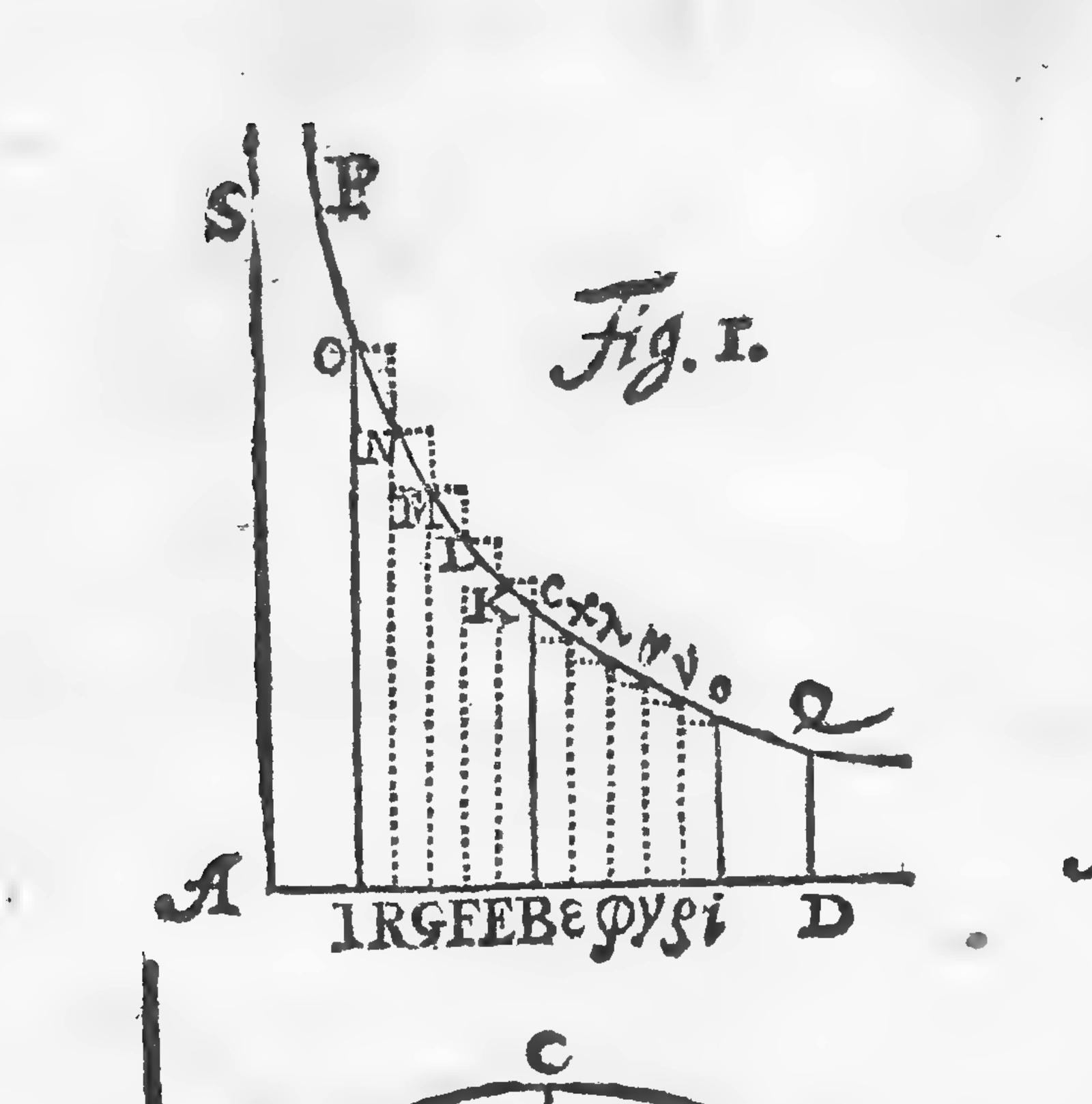
Figure 1.3. Compound interest, drawn in 1713. Read the base line right to left: the ordinate at B is the principal, and at each of the equal moments E, F, G the sum is struck again, so that BC, EK, FL, GM climb in continued proportion to the terminal ordinate IO. Measuring the engraving, those successive heights stand in ratios of about 1.13, 1.15 and 1.15 — roughly constant, as continued proportion requires, on a plate drawn by hand. Bernoulli then makes the number of moments infinite: the chord “passes into the tangent, and t into the subtangent of the logarithmic curve.” That subtangent is the reciprocal of what we now call the force of interest, and the terminal ordinate is e^r. Source: Jakob Bernoulli, Tractatus de seriebus infinitis, Prop. LIX and Scholium, pp. 303–304, with Fig. 1 on the plate “Ad pag. 306,” bound with Ars Conjectandi (Basel, 1713); Smithsonian Libraries copy, public domain.

Bernoulli’s own cross-reference, “Conf. Act. Lips. 1690 p. 222,” points back to the Acta Eruditorum of 1690, where he had first posed the problem. The Latin reads almost as a caption for a figure one is meant to manipulate: divide the year more finely, and watch the polygon of chords flatten onto the curve. It took another century and a half for the picture to reach a textbook.

¹ Jakob Bernoulli, “Quaestiones nonnullae de usuris, cum solutione problematis de sorte alearum, propositi in Ephem. Gall. A. 1685,” Acta Eruditorum (Leipzig), May 1690, pp. 219–223 — where the continuous-compounding question is posed and the limit shown to fall between 2 and 3. The pairing is characteristic: a question about interest answered alongside a problem about dice from the Journal des Sçavans of 1685, by the man who would go on to write the Ars Conjectandi. Bernoulli sends the reader back to this article himself — the 1713 Scholium closes “Conf. Act. Lips. 1690 p. 222,” a page inside it. ↩

The actuary William Sutton drew it again in the Institute of Actuaries’ text-book of 1882 — this time in the orientation we still use, with growth running to the right of the origin and present values falling away to the left.

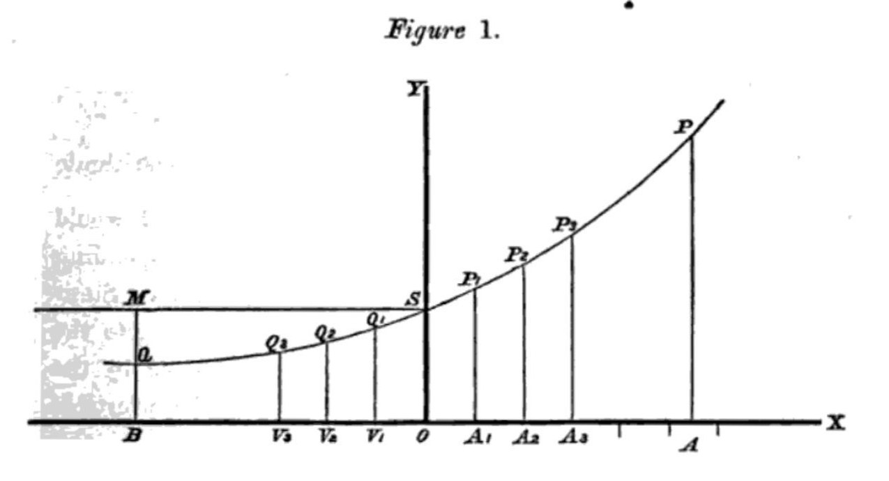
William Sutton's 1882 figure of the compound-interest curve: the accumulation of 1 to the right of the origin, present values to the left

Figure 1.4. The compound-interest curve in its modern orientation. To the right of the origin the ordinate PA is the amount to which 1 grows over the time OA at rate i; to the left, QB is the present value of 1 — the same curve run in both directions, a century and a half before the interactive above — and 169 years after Bernoulli. Source: William Sutton, Institute of Actuaries’ Text-Book, Part I (London, 1882), Fig. 1; public domain.

Discounting Is Perspective

Here is a picture I like to draw for it. Imagine driving a long, straight highway across the desert toward a distant range of mountains. Billboards line the road. The one you are passing looms enormous; the next is smaller; the ones near the horizon have shrunk to postage stamps. Now suppose each billboard is a dollar you have been promised — one now, one in five years, one in ten, and so on down the road. The far ones look smaller for the very reason they are worth less: distance. The interest rate is simply how fast the billboards shrink as they recede — a high rate is a steeply narrowing road that dwindles the far dollars almost to nothing, a low rate a gentle perspective in which even distant dollars stay nearly full size.

Figure 1.3. Discounting as perspective. Picture driving a desert highway toward the horizon; each billboard is a dollar you have been promised — one now, and the rest at five-year intervals down the road. The far ones look smaller for exactly the reason they are worth less: distance. Here the rate is 5% a year, so the dollar due in twenty years has shrunk to about thirty-eight cents. The interest rate is simply how fast the billboards dwindle as they recede.

That is the whole idea, and the rest of the book is built on it. The price of a bond is the discounted value of its coupons and principal; the value of a stock is the discounted value of its future dividends; the return an investor demands is precisely the rate that makes a security’s distant dollars worth its price today. So before we turn to risk and reward, keep the highway in mind: money has a time dimension, and comparing money across time means bringing it back down the road to what it is worth today.

II. Finance from the Investor's Perspective

This book takes the perspective of the investor. We examine how shareholders and bondholders who hold portfolios — collections of different securities — make financial decisions. The central question addressed is:

What rate of return will investors demand to hold a risky security?

That single question — how much extra return investors demand as compensation for risk — runs through the whole book, and this chapter does not yet fully answer it. It takes the first steps: defining return, measuring the historical record, and naming the reward for bearing risk (the risk premium, Section VII). The complete answer — how the market itself sets the price of risk — is built over the chapters that follow, through diversification and the efficient frontier and the asset-pricing models beyond. Keep the question in view: nearly every tool in this text is, in the end, an attempt to answer it.

III. Why Investors Invest

Why part with money you could enjoy spending today? The reason is nearly always the same: you expect to need it later. Every dollar saved is current consumption deferred, and consumption is deferred only for a reason — some future need. Retirement, a child’s education, a home, a cushion against emergencies, a gift or a bequest, an institution’s obligations decades away: each is a claim the future will make on you, and saving is how you prepare to meet it.

Investing, then, is really an exercise in planning. It means identifying the future needs that matter to you, judging what they will cost and when they will fall due, and allocating today’s assets among investments whose expected future value lines up with those needs. This is what the time value of money is for. It is what makes the plan possible — because money invested grows, a smaller sum set aside now can meet a larger need later — and it is what makes the plan necessary, since needs arriving at different dates must be compared, discounted, and funded from the resources you hold today.

The great institutional investors are simply this logic written large. A pension fund invests to meet the retirements it has promised; a university endowment, to sustain its spending in perpetuity; a sovereign wealth fund, to turn a country’s finite oil into income for generations not yet born. Each is a pool of present assets deliberately arranged to satisfy a schedule of future needs. Households do the same on a smaller scale, whether or not they put it in those words.

Other motives exist. Some buy a long-shot security for the thrill of an outside chance; some invest for charitable ends whose rewards are never financial. Still, the central and near-universal reason people hold securities is to move purchasing power from the present, where they have more than they need, to the future, where they expect to need more than they will have.

IV. Definition of Rates of Return

Return is the growth in wealth an investment produces, expressed as a percentage so that investments of any size can be compared. The basic formula measures the change in price relative to what you paid — click any part of the equation to see what it does:

R_t = P_t+1 − P_t P_t = P_t+1P_t − 1

👈 click a term — the choice of denominator is the subtle, powerful one

Click a term in the equation above to see what it means.

That denominator is worth pausing on. Dividing by the original price is what turns a dollar gain into a rate — a number that means the same thing whatever the sum invested, and so can be compared across investments of any size. This small step is what makes return generalizable across investments of any size.

Most securities also pay cash along the way. Adding those dividends to the price change gives the total return:

R_t = P_t+1 − P_t + D_t P_t

Click the added term to see what changed.

V. Arithmetic vs. Geometric Rates of Return

Over many periods there are two ways to average returns, and they answer different questions. Click through each formula to see what it is really doing:

R_A = 1T ∑_t=1^T R_t

👈 click a term to name it

Click a term above.

R_G = [ ∏_t=1^T (1 + R_t) ]^1/T − 1

👈 complicated on the surface — tap each piece and it comes apart into four simple ideas

Click any piece of this one — growth factor, product, root, minus one.

Consider an illustrative example: $P_0 = \$100$, $R_1 = -50\%$, $R_2 = +100\%$. After the first period, wealth falls to $50; after the second, it returns to $100. The arithmetic average return is $\frac{-50\% + 100\%}{2} = 25\%$, but the geometric average is $\sqrt{(0.50)(2.00)} - 1 = 0\%$.

Key Concept: Arithmetic vs. Geometric Returns

The geometric return better reflects the actual investment experience (compound growth), while the arithmetic return suits single-period statistical models. The geometric mean is always less than or equal to the arithmetic mean, with the gap increasing as volatility rises.

Side Note: Stock Returns over the Very, Very Long Term

Before we turn to a century of U.S. data, it is worth zooming out. A century is a long record by modern standards, but one company gives us six. Along the Garonne at Toulouse, a company of grain mills known as the Bazacle divided its ownership into transferable shares — the uchaux — as early as the twelfth century. From 1372 until the firm was nationalized in 1946 it kept registers of share transactions and dividends that survive almost unbroken: the longest continuous record of a traded stock we possess — nearly six hundred years of prices and payouts, measured in constant grams of silver.

The Bazacle on the Garonne at Toulouse. The milling company whose shares traded here for nearly six centuries still harnesses the river’s current — the site now houses a hydroelectric station.

What that record shows is striking. Over the very long run the Bazacle behaved as an income stock rather than a growth stock. In real terms the share price barely moved across the centuries; almost the whole return came from a steady dividend yield of about 5.5% a year rather than from rising prices. Yet the price still tracked the discounted value of expected future dividends remarkably faithfully through war, plague, revolution, and inflation — the present-value relation at work over a horizon no modern market can offer. It is a useful counterpoint to the U.S. century that follows, where most of the return came from compounding price growth.

Le Bris, D., W. N. Goetzmann, and S. Pouget. “The Present-Value Relation over Six Centuries: The Case of the Bazacle Company.” Journal of Financial Economics 132 (2019). Explore the full series in the Origins of the Corporation interactive.

VI. A Century of U.S. Asset Returns

Over the full century from 1926 through 2025, a dollar invested in large-cap U.S. stocks (the S&P 500 and its predecessors) grew to roughly $14,750 — and a dollar in small-cap stocks to about $32,400 — while a dollar in long-term government bonds grew to only about $117, and in 30-day Treasury bills to about $25. Over the same span consumer prices rose roughly eighteen-fold. The stock lines display far greater volatility than the bond lines, but the terminal-wealth difference is enormous — the power of compounding a higher average return over a long horizon.

Data note: Figures and tables in this chapter are computed from the Stocks, Bonds, Bills, and Inflation (SBBI) series of annual and monthly U.S. capital-market returns, 1926–2025 — the modern extension of the historical record assembled by Roger G. Ibbotson and Rex A. Sinquefield. See the sidebar below.

Sidebar: Fifty Years of Stocks, Bonds, Bills, and Inflation

In 1976 Roger G. Ibbotson and Rex A. Sinquefield published a pair of papers in the Journal of Business that gave the profession its first careful, long-horizon accounting of U.S. capital-market returns — the year-by-year historical returns on stocks, bonds, bills, and inflation back to 1926, together with a companion paper simulating their future distribution. Half a century later, the acronym they coined — SBBI — is still the standard shorthand for the historical record, and the annual yearbook built on it became a fixture on every investment professional’s shelf.

The data used throughout this textbook extend that record through year-end 2025, drawn from the revised SBBI series prepared for Roger G. Ibbotson’s forthcoming volume, Exponential Wealth: Centuries of Stock and Bond Returns (CFA Institute Research Foundation, forthcoming 2026). The year 2026 marks the fiftieth anniversary of the original Ibbotson–Sinquefield publications.

Ibbotson, R. G., and R. A. Sinquefield. “Stocks, Bonds, Bills, and Inflation: Year-by-Year Historical Returns (1926–1974).” Journal of Business 49, no. 1 (1976): 11–47; and “… Simulations of the Future (1976–2000).” Journal of Business 49, no. 3 (1976): 313–338.

Growth of $1 invested in stocks vs bonds, 1926 to 2025

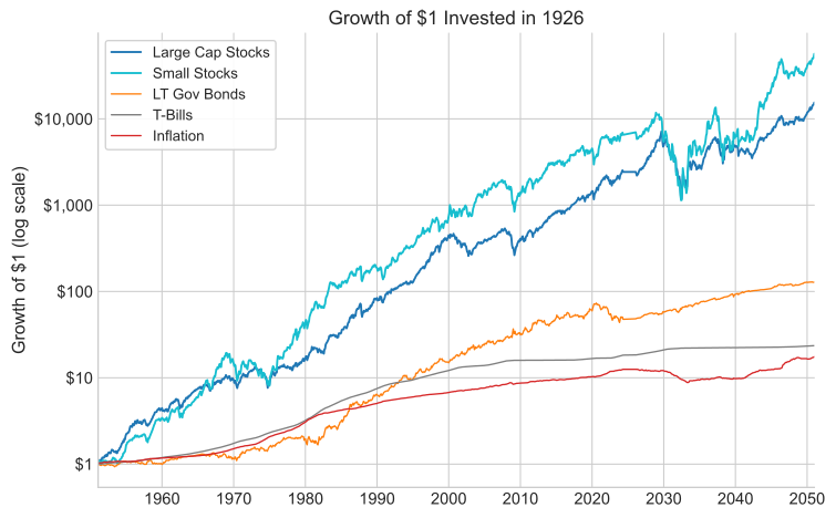
Figure 1.4. Growth of $1 invested in U.S. stocks, bonds, and Treasury bills (1926–2025, log scale). Computed from SBBI data. Stocks dramatically outperform bonds over long horizons, but with substantially greater year-to-year volatility.

VII. The Risk Premium

The return differential between stocks and bonds is attributed to risk differences. "Volatility" describes the shakier performance of stocks compared to bonds. Investors are risk-averse — they prefer less risk when other factors remain equal. This motivates the concept of the risk premium: the additional return demanded for holding risky securities versus riskless alternatives like Treasury Bills.

Equity Premium

$$\text{Equity Premium} = \bar{R}_{\text{stocks}} - \bar{R}_{\text{T-bills}}$$

From 1926–2025, the equity premium (large-cap stocks over 30-day Treasury bills) was approximately 8.5% (arithmetic) or 6.8% (geometric) annually.

Summary Statistics (1926–2025)

Investment	Geometric Mean	Arithmetic Mean	Std. Dev.	High Return	Low Return
Large-Cap Stocks (S&P 500) TR	10.07%	11.85%	19.04%	49.9%	−43.3%
U.S. Small-Cap Stocks TR	10.95%	14.44%	27.69%	115.7%	−50.1%
LT Govt. Bonds (20Y) TR	4.88%	5.40%	10.62%	41.8%	−27.2%
IT Govt. Bonds (5Y) TR	4.84%	5.00%	5.91%	29.7%	−9.5%
U.S. 30-day T-Bills	3.26%	3.30%	3.09%	15.1%	−1.7%
Inflation (CPI)	2.94%	3.01%	3.92%	18.1%	−10.3%

Source: SBBI series, 1926–2025 (Ibbotson, Exponential Wealth, forthcoming 2026). High/Low columns are the best and worst single calendar-year total returns.

VIII. Standard Deviation as a Measure of Risk

Standard deviation quantifies volatility mathematically as the square root of the variance. It calculates the average spread of observations around the mean:

Standard Deviation

$$\sigma = \sqrt{\frac{1}{T-1}\sum_{t=1}^{T}\left(R_t - \bar{R}\right)^2}$$

For large-cap stock returns (approximately $\sigma = 19.0\%$), assuming a normal distribution, approximately two-thirds of observations should fall within one standard deviation of the mean:

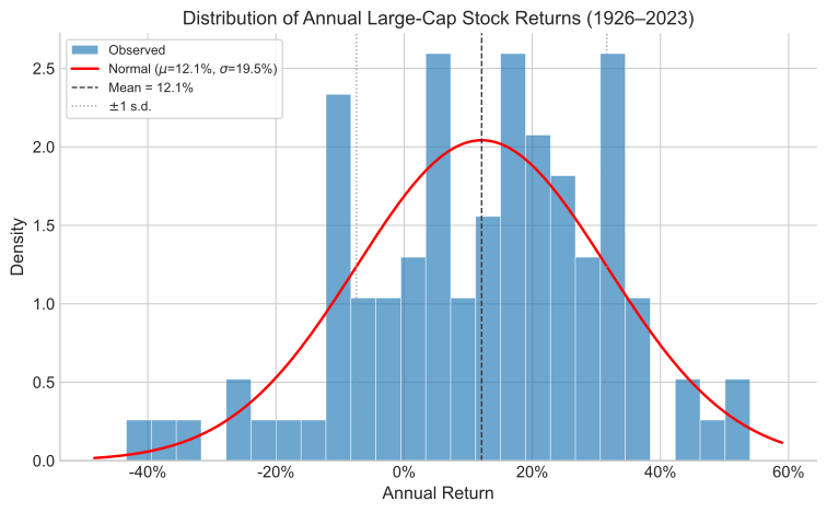
$$\bar{R} \pm \sigma \approx 11.85\% \pm 19.0\% = [-7.2\%,\; 30.9\%]$$

Figure 1.5. Distribution of large-cap stock annual returns (1926–2025), computed from SBBI data. The histogram shows the ±1 standard deviation range containing roughly 68% of observations. Actual return distributions exhibit "fatter tails" than the normal distribution predicts.

Limitations of Standard Deviation

The chapter acknowledges several limitations:

Standard deviation equally weights high and low returns
It heavily weights extreme observations
It ignores distribution shape (skewness and kurtosis)

However, the benefits include providing a single comparable risk measure enabling portfolio analysis decisions.

There is evidence that stock returns may follow "stable" distributions with undefined variance rather than normal distributions, a hypothesis advanced by Benoit Mandelbrot. Return distributions show "fatter tails" than log-normal predictions suggest — extreme events (both positive and negative) occur more frequently than a normal model predicts.

Key Concept: Standard Deviation as Risk

Standard deviation provides a single, comparable measure of risk that enables systematic portfolio analysis. Despite its limitations — especially its assumption of symmetric, normally distributed returns — it remains the foundational risk measure in modern portfolio theory.

IX. Risk and the Investment Horizon

The standard deviation measures risk over a single period. But investors hold for many periods, and over a long horizon the picture splits in two. Suppose returns follow a random walk — each year’s return independent of the last. Then two kinds of uncertainty scale in opposite directions as the horizon lengthens. Uncertainty about your ending wealth grows, because independent shocks accumulate and the range of possible fortunes fans out as the square root of time. But uncertainty about your average annual return shrinks, because averaging over more years cancels the noise and the estimate closes in on the true mean — again as the square root of time. The figure below lets you watch both at once.

Mean return: 7% Volatility: 18%

Figure 1.6. Two faces of the random walk. Each faint line is one simulated 40-year history of a dollar earning a random annual return (mean and volatility set by the sliders); the shaded bands are the theoretical 68% and 95% ranges. The trumpet: uncertainty about ending wealth fans out with the square root of time — the longer the horizon, the wider the spread of fortunes. The tulip (toggle): uncertainty about the average annual return does the opposite, narrowing as one over the square root of time, closing in on the true mean. More time makes the destination less certain and the average more certain — two faces of the same square-root-of-time law.

The lesson is subtle and important. Give the market enough time and you can pin down what its average return has been to within a fraction of a percent — the tulip narrowing. Yet the same random walk guarantees that where any single dollar actually ends up stays highly uncertain, however long you wait — the trumpet widening. It is why we can speak with confidence about the historical equity premium, and yet no one can tell you what your retirement account will be worth in forty years.