Chapter IV
The Portfolio Approach to Risk
The Capital Asset Pricing Model, Two Fund Separation, and the meaning of portfolio risk.
I. The Quest for the Tangency Portfolio
In the 1960s, financial researchers working with Harry Markowitz's mean-variance model of portfolio construction made a remarkable discovery that would change investment theory and practice in the United States and the world. The discovery was based upon an idealized model of the markets, in which all the world's risky assets were included in the investor opportunity set and one riskless asset existed, allowing both more and less risk-averse investors to find their optimal portfolio along the tangency ray.
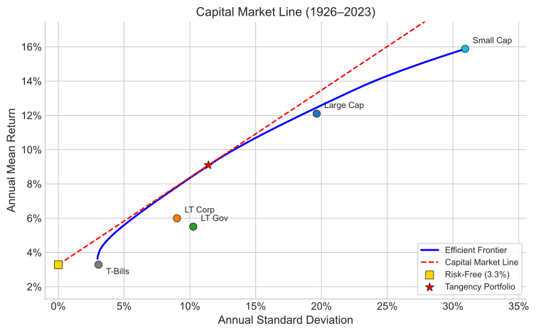
Figure 4.1. Two Fund Separation, computed from SBBI data. All investors hold the same tangency portfolio $T$ of risky assets. More risk-averse (MRA) investors mix $T$ with T-bills; less risk-averse (LRA) investors borrow at $R_f$ to lever up their position in $T$.
Assuming that investors could borrow and lend at the riskless rate, this simple diagram suggested that everyone in the world would want to hold precisely the same portfolio of risky assets! That portfolio, identified at the point of tangency, represents some portfolio mix of the world's assets. Identify it, and the world will beat a path to your door.
Key Concept: Two Fund Separation Theorem
The tangency portfolio became the centerpiece of a classical model in finance. The "Two Fund Separation Theorem" argues that all investors will make their choice between two funds: the risky tangency portfolio and the riskless "fund." Every investor holds the same risky portfolio — they differ only in leverage.
Identifying this tangency portfolio is harder than it looks. Recall that a major difficulty in estimating an efficient frontier accurately is that errors grow as the number of assets increase. You cannot just dump all the means, standard deviations, and correlations for the world's assets into an optimizer and turn the crank. If you did, you would get a nonsensical answer. Sadly enough, empirical research was not the answer, due to statistical estimation problems.
The answer to the question came from theory. Financial economist William Sharpe is one of the creators of the "Capital Asset Pricing Model," a theory which began as a quest to identify the tangency portfolio. Since that time, it has developed into much, much more. In fact, the CAPM, as it is called, is the predominant model used for estimating equity risk and return.
II. The Capital Asset Pricing Model
Because the CAPM is a theory, we must assume for argument that:
- All assets in the world are traded
- All assets are infinitely divisible
- All investors in the world collectively hold all assets
- For every borrower, there is a lender
- There is a riskless security in the world
- All investors borrow and lend at the riskless rate
- Everyone agrees on the inputs to the Mean-STD picture
- Preferences are well-described by simple utility functions
- Security distributions are normal, or at least well described by two parameters
- There are only two periods of time in our world
This is a long list of requirements, and together they describe the capitalist's ideal world. Everything may be bought and sold in perfectly liquid fractional amounts — even human capital! There is a perfect, safe haven for risk-averse investors, i.e. the riskless asset. This means that everyone is an equally good credit risk! No one has any informational advantage in the CAPM world. Everyone has already generously shared all of their knowledge about the future risk and return of the securities, so no one disagrees about expected returns. All customer preferences are an open book — risk attitudes are well described by a simple utility function. There is no mystery about the shape of the future return distributions. Last but not least, decisions are not complicated by the ability to change your mind through time. You invest irrevocably at one point, and reap the rewards of your investment in the next period — at which time you and the investment problem cease to exist. Terminal wealth is measured at that time.
He who dies with the most toys wins! The technical name for this setting is "a frictionless one-period, multi-asset economy with no asymmetric information."
The CAPM argues that these assumptions imply that the tangency portfolio will be a value-weighted mix of all the assets in the world.
The Equilibrium Proof
The proof is an elegant equilibrium argument. It begins with the assertion that all risky assets in the world may be regarded as "slices" of a global wealth portfolio. We may graphically represent this as a large, square "cake," sliced horizontally in varying widths. The widths are proportional to the size of each company — determined by the number of shares times the price per share.
Figure 4.2. The CAPM equilibrium argument. The global wealth "cake" can be sliced by company (horizontally) or by investor (vertically). Since all investors hold the same risky portfolio weights, each vertical slice has the same proportions. The weights equal each company's share of total world wealth.
Here is the equilibrium part of the argument: Assume that all investors in the world collectively hold all the assets in the world, and that, for every borrower at the riskless rate there is a lender. This last condition is needed so that we can claim that the positions in the riskless asset "net out" across all investors.
From the two-fund separation picture, we already know that all investors will hold the same portfolio of risky assets, i.e. that the weights for each risky asset $j$ will be the same across all investor portfolios. This knowledge allows us to cut the cake in another direction: vertically. As with companies, we vary the width of the slice according to the wealth of the individual.
Notice that each vertical "slice" is a portfolio, and the weights are given by the relative asset values of the companies. We can calculate what the weights are exactly:
CAPM Portfolio Weight
$$w_i = \frac{P_i \times N_i}{W_{\text{world}}}$$where $P_i$ is the price of asset $i$, $N_i$ is the number of shares, and $W_{\text{world}}$ is total world wealth. Each investor's portfolio weight is exactly proportional to the percentage that the firm represents of the world's assets.
Key Concept: The CAPM Result
The tangency portfolio is a capital-weighted portfolio of all the world's assets. This is not an empirical finding — it is a theoretical conclusion that follows from the equilibrium assumptions. Every investor holds the "market portfolio."
III. Investment Implications
The CAPM tells us that all investors will want to hold "capital-weighted" portfolios of global wealth. In the 1960s when the CAPM was developed, this solution looked a lot like a portfolio that was already familiar to many people: the S&P 500. The S&P 500 is a capital-weighted portfolio of most of the U.S.'s largest stocks. At that time, the U.S. was the world's largest market, and thus, it seemed to be a fair approximation to the "cake."
Amazingly, the answer was right under our noses — the tangency portfolio must be something like the S&P 500!
Not coincidentally, widespread use of index funds began about this time. Index funds are mutual funds and/or money managers who simply match the performance of the S&P. Many institutions and individuals discovered the virtues of indexing:
- Minimal trading costs: Capital-weighted portfolios automatically adjust to changes in value when stocks grow, so investors need not change their weights all the time — it is a "buy-and-hold" portfolio
- Competitive performance: There was little evidence at the time that active portfolio management beat the S&P index — so why not simply index?
IV. Is the CAPM True?
Any theory is only strictly valid if its assumptions are true. There are a few nettlesome issues that call into question the validity of the CAPM:
- Is the world in equilibrium?
- Do you hold the value-weighted world wealth portfolio?
- Can you even come close?
- What about "human capital?"
While these problems may violate the letter of the law, perhaps the spirit of the CAPM is correct. That is, the theory may be a good prescription for investment policy. It tells investors to choose a very reasonable, diversified and low-cost portfolio. It also moves them into global assets, i.e. towards investments that are not too correlated with their personal human capital. In fact, even if the CAPM is approximately correct, it will have a major impact upon how investors regard individual securities. Why?
V. Portfolio Risk
Suppose you were a CAPM-style investor holding the world wealth portfolio, and someone offered you another stock to invest in. What rate of return would you demand to hold this stock? The answer before the CAPM might have depended upon the standard deviation of a stock's returns. After the CAPM, it is clear that you care about the effect of this stock on the tangency portfolio.
The introduction of asset $A$ into the portfolio will move the tangency portfolio. The extent of this movement determines the price you are willing to pay (alternately, the return you demand) for holding asset $A$. The lower the average correlation $A$ has with the rest of the assets in the portfolio, the more the frontier — and hence $T$ — will move to the left. This is good news for the investor: if $A$ moves your portfolio left, you will demand lower expected return because it improves your portfolio risk-return profile.
Key Concept: Why it's Called the Capital Asset Pricing Model
The CAPM explains relative security prices in terms of a security's contribution to the risk of the whole portfolio, not its individual standard deviation. What matters is not how volatile a stock is on its own, but how it co-moves with the market. This co-movement is measured by beta ($\beta$).
The CAPM pricing relationship can be expressed as:
The CAPM Equation
$$E(R_i) = R_f + \beta_i \left[E(R_M) - R_f\right]$$where beta measures the sensitivity of asset $i$'s return to the market return:
Beta
$$\beta_i = \frac{\text{Cov}(R_i, R_M)}{\text{Var}(R_M)} = \frac{\sigma_{iM}}{\sigma_M^2}$$Figure 4.3. The Security Market Line (SML). Expected return is a linear function of beta — a security's contribution to portfolio risk. Securities above the line are undervalued (positive alpha); those below are overvalued.
Use it as a hurdle rate. Read a security's beta off the horizontal axis and the line returns the rate it must earn to be worth holding — the benchmark you discount its cash flows against. A security plotting above the line is underpriced (positive alpha); below it, overpriced. The research tool just below lets you build a book and measure that alpha on live data.
The four lenses for reading each picture ↗This picture, too, is older than it looks. Its first drawing was William Sharpe’s, in his 1961 doctoral thesis — and, like Markowitz’s frontier, he drew it with the axes the other way around: his risk measure B (the ancestor of beta) up the vertical, expected return E along the horizontal, and the line cutting the return axis at the pure interest rate.
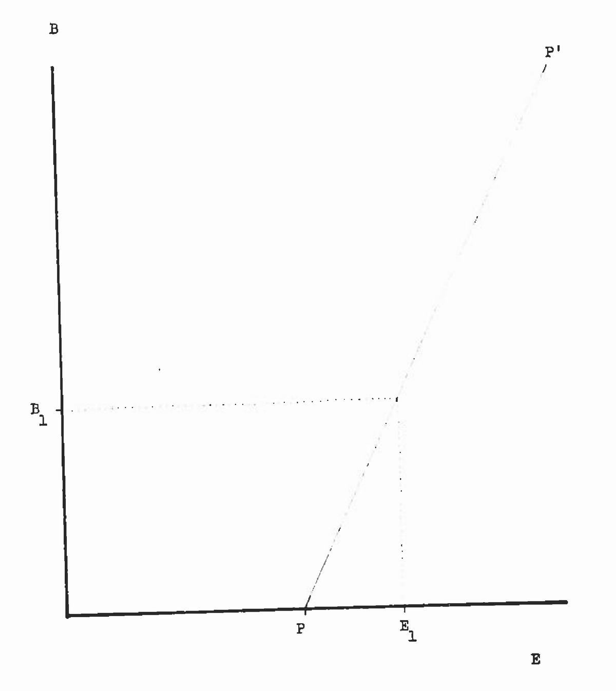
Sharpe’s original Security Market Line. On the left, Figure 24 as it appears in the thesis — drawn by hand, the sloping line laid in as a row of dots. On the right the same construction redrawn, because the original is faint. In equilibrium every security lies on one straight line: its risk B and its expected return E rise together, and the line meets the E-axis at P, the pure interest rate — the return on a riskless, zero-risk security. A security in equilibrium sits at E1, B1. From W. F. Sharpe, Portfolio Analysis Based on a Simplified Model of the Relationships Among Securities (Ph.D. dissertation, UCLA, 1961), Fig. 24. Its axes are transposed from the modern convention above — the same “old-convention” tell as Markowitz’s first frontier.
Build Your Own Long-Short Book
The line is not just a picture — it is a tool. Enter up to eight tickers and weights (negative to short); the figure fetches five years of monthly prices, regresses each stock on the market for its beta and alpha, and plots them against the SML. Dots above the line beat what their beta warranted (positive alpha); dots below fell short. The reward for combining them is the information ratio — alpha per unit of the diversifiable risk you carry — and the figure shows both its estimate and how little we should trust it.
Figure 4.4. The Security Market Line as a research tool. Each dot is a stock at its estimated beta (horizontal) and realized annual return (vertical); the line is the SML from the risk-free rate through the market. Green dots sit above it (positive alpha), red below; dot size is the weight. The portfolio itself is the blue diamond — plotted at its own beta and return, so its alpha is the gap from the line, just like each stock. The readout gives the information ratio — portfolio alpha over residual risk computed from the full residual covariance matrix — with a 95% band of $\pm 1.96/\sqrt{\text{years}}$ and a “noise floor” $\sqrt{N/\text{years}}$, the in-sample IR a skill-less book of $N$ names produces by chance (Grinold & Kahn). Tick shrink alphas for the honest expected IR once estimation error is removed. Live data via Yahoo Finance.
VI. Conclusion
The CAPM is a theoretical solution to the identity of the tangency portfolio. It uses some ideal assumptions about the economy to argue that the capital-weighted world wealth portfolio is the tangency portfolio, and that every investor will hold this same portfolio of risky assets. Even though it is clear they do not, the CAPM is still a very useful tool. It has been taken as a prescription for the investment portfolio, as well as a tool for estimating an expected rate of return.
The CAPM's practical legacy is enormous:
- It provided the intellectual foundation for index fund investing
- It shifted focus from individual stock volatility to portfolio contribution (beta)
- It established the Security Market Line as a benchmark for evaluating investment performance (alpha)
- It remains the predominant model for estimating equity cost of capital in corporate finance